Simple Logistic Regression, with which treatment will we have more probability of cured animals?
In this article, we are going to address a regression technique that allows us to relate a categorical dependent variable (for example cured/non cured) with one or more quantitative and/or categorical independent variables. This is the logistic regression.
We will focus on simple binary logistic regression, which relates a dichotomous dependent variable (two options) and an independent variable.
What is logistic regression?
The objective of this statistical technique is to express the probability that an event occurs depending on certain variables, which are considered potentially influential. We will have a categorical dependent variable, which can be dichotomous or polytomous, and one or more quantitative and/or categorical independent variables.
A dichotomous dependent variable has only two possible answers: yes or no, true or false, sick or not sick, cured or not cured, success or failure. These responses are coded with a value of 1 if a certain event occurs or with a value of 0 if this event does not occur. This aspect of the coding of the variables is not trivial, it influences the way in which the mathematical calculations are carried out and we must take it into account when interpreting the results.
In this type of process in which there are only two possible outcomes (0/1), the probability of each outcome being constant over a series of repetitions is distributed under the binomial law.
The simple logistic regression is a statistical test used to predict a single binary variable using one other variable.
The problem and solution using a simple logistic regression
Let us see with a practical example how to perform and interpret a simple logistic regression model.
We are going to check the effectiveness of two alternative treatments on the cure of a disease.
The objective is to study whether the cure/non-cure process is associated with the treatment or not. In other words, we are testing if the probability of cure applying treatment A is equal to, or different from, the probability of cure applying treatment B.
To do this, suppose that we have performed an experiment on a random sample of 40 sick animals, randomly divided into two groups of 20 animals, each of which is given a treatment (A or B). The results obtained in the experiment are shown in the following table:
| Treatment A (X = 1) | Treatment B (X = 0) | |
|---|---|---|
| Cure (Y = 1) | 18 | 13 |
| Non-cure (Y = O) | 2 | 7 |
Before proposing a logistic regression model, we can make a series of calculations:
We can estimate the probability of cure (p) for both treatments:
- Treatment B (0.65): p | (X = 0) = 13/20;
- Treatment A (0.90): p | (X = 1) = 18/20
In: p | (X = 0) = 13/20, p is the healing chance.
| is a symbol that means “conditioned on”.
X = 0 indicates that the data belong to the animals assigned to treatment B.
Therefore, the probability of cure for the animals that received treatment B is 65%.
As both probabilities are numerically different, it could seem that the probability of cure depends on the treatment. But before reaching this conclusion, we should ask ourselves two questions: is this dependency generalizable (“statistically significant”)? And how much does the response depend on the treatment (“clinically relevant”)?
In this example, we could also respond from the data in the table by applying the concepts of odds and odds ratio that we explain in the articles of case-control studies in epidemiology (available in Spanish):
- Odds with treatment B = (13/20)/(7/20). Applying treatment B there are 1.857 more probabilities of cure than of non-cure.
- Odds with treatment A = (18/20)/(2/20). Applying treatment A there are 9 more probabilities of cure than of non-cure.
- Odds ratio OR = odds.treatment.B/odds. treatment A. Applying treatment A there are 4.846 (≈5) more chances of cure than with treatment B
In case there were no differences, odds and OR would be 1.
These values are point estimates and therefore, we must also use their confidence interval to indicate the precision of the estimate. Thus, we cannot yet conclude that the probability of cure depends on the treatment.
Simple logistic regression with Síagro
To perform this analysis, we have used the software Síagro and a database with the following information:
| id | cure | treatment |
| 1 | 1 | 0 |
| 2 | 1 | 0 |
| 3 | 1 | 0 |
| . | . | . |
| . | . | . |
| . | . | . |
| 38 | 1 | 1 |
| 39 | 0 | 1 |
| 40 | 0 | 1 |
The first thing we have done is log into the application, load our Excel file and access the Prediction / Logistics Models in the control panel.
Both cure or non-cure (dependent variable) and treatment (independent variable) are variables that follow a binomial distribution, but we don’t have to worry about remembering or telling the Síagro software because it already knows.
If we select our variables in the dashboard:
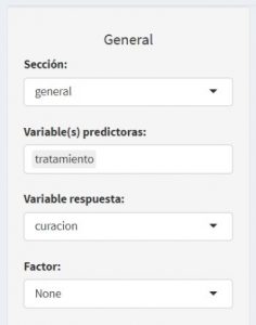
We obtain the following results:
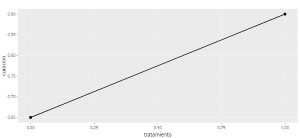
| term | estimate | std.error | statistic | p.value | Sig |
| (Intercept) | 0.619 | 0.469 | 1.32 | 0.187 | |
| treatment | 1.58 | 0.88 | 1.79 | 0.0731 | . |
| null.deviance | df.null | logLik | AIC | BIC | deviance | df.residual | nobs |
| 42.7 | 39 | -19.5 | 42.9 | 46.3 | 38.9 | 38 | 40 |
How do we interpret this output?
Firstly, the chart explains the relation between two variables and it is a straight line because it is a linear model.
Estimate: is the estimation of the coefficients:
- Intercept, origin, is the estimation of the coefficient a (0,6190), which coincides with the natural logarithm of the odds when X = 0
- treatment is the estimation of the coefficient b (1.578) which is the natural logarithm of OR.
From the coefficients a and b we can calculate the odds when X = 0 and the OR would be:
- exp(a)=exp (0,619)= 1,857 = odds for X = 0.
- Exp(b)=exp (1,5784)= 4,846 = OR
Std.error is the standard error of the coefficients.
Statistic or Z value is the contrast statistic. Z is the distance from the mean relative to the standard deviation of the mean. It is calculated from the ratio between the coefficient and its standard error to obtain the p-value (Pr(>|z|)) shown below. Just as in the comparison of means, the student’s test was used and a “t” statistic was calculated, for this analysis the statistic used is “z”.
P.value (the Pr(>|z|) are the p values that indicate whether the coefficients are significantly different from zero or not (given a level of significance that we establish at p<0.05). We must take into account that studying whether the values of a and b are significantly different from 0, or not, is equivalent to studying whether exp(a) (odds for treatment B) and exp(b) (OR) are significantly different from 1.
The Intercept, Pr (>|z|)=0.187, means that there is no significance, and we cannot say that a is significantly different from zero. In this case, this statement also corresponds to the fact that exp(a), that is, the odds for X = 0 (treatment B), is not significantly different from 1 (because exo(0)=1).
As a consequence, we say that for the animals in treatment B, the probability of cure is equal to that of no cure.
Similarly, in the row treatment, Pr(>|z|)=0.073; As the level of significance is 0.05, we did not find significance either, so the conclusion is that exp(b) is not significantly different from 1.
This represents that there are no differences in the probability of cure between treatments A and B.
As we have seen, this software allows users to obtain complete analysis and answer such a complex question in just a few clicks.
